Problem Statement#
Our goal was to create a deep learning model that would accurately predict daily Covid-19 cases. To achieve this, we used a multivariate, multi-horizon approach that integrates heterogeneous types of inputs for each county.
Our prediction model, \(f(.)\) was defined as:
\(\hat y_i(t, \tau) \) represents the predicted number of cases in a day at a given time \(t \in [0, T_i] \) for any county \(i\), with \tau as days into the future, and \(T_i\) as the length of the time series period. In our study, we use the previous 13 days of data to forecast the next 15 days of data —- this is where the multi-horizon approach comes in. Our approach employs the Temporal Fusion Transformer (TFT) as the primary time-series model, which we discuss in the next chapter. Besides examining how the model performs against the ground truth, we wish to understand the model’s inner workings and interpretability through attention-based analysis.
Data Model Preparation#
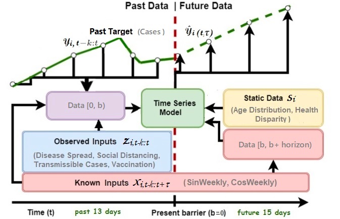
Fig. 1 provides a high-level overview of the data model preparation for our research:

As shown in the image above, we feed three types of covariates at inputs into the time series model, using the past 13 days to predict the next 15 days of time series data.
These three types of inputs are:
Static Inputs : Each county i is associated with a set of static inputs \(s_i\), which do not vary over time and are specific to that county’s demographics.
Observed or Past Inputs : Observed inputs are time-varying features known at each timestamp \(t \in [0, T_i]\) (e.g., Vacciation, Disease Spread, Social Distancing, Transmissible Cases), but their future values are unknown. We incorporate all past information within a lookback window of k (the past 13 days), using target (cases) and observed inputs upto the forecast start time t: \(\space y_{i,t-k:t} = {y_{i,t-k}, ..., y_{i, t} }\) and \(z_{i, t-k:t} = {z_{i,t-k}, ..., z{i, t}}\).
Known Future Inputs: These inputs $x_{i, t} can be measured beforehand, which in our case are the sine and cosine of the day of a week at a given date, and are known at the time of prediction. We also add known future inputs across the entire range for the TFT.
